In 2010, Edward Witten delivered a lecture to the general public on behalf of IAS (Institute for Advanced Studies in the USA) on entanglement theory and quantum mechanics. In this article we will convey the main points of his words with specific extensions. On the face of it, nexus theory began as another mathematical "trick", but like most scientific discoveries, the mathematicians preceded the physicists by several decades

Tying and priming are routine operations. Every day many of us tie our shoelaces in order to allow the shoelace to do its job - to firmly connect the sides of the shoe. From time to time the connection comes to our detriment - who among us has not experienced the feeling of frustration when he discovered that the wired headphones in his pocket were tangled together or that the delicate piece of jewelry he had just bought naturally twisted and formed tight bonds. The challenge, of course, is to unravel the ties, which requires a lot of effort and a lot of time.
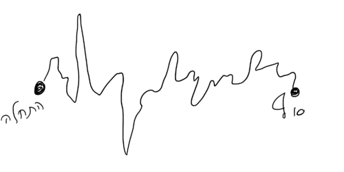
For the mathematicians, the term "connection" is more abstract but all in all it describes a loop that floats freely in space-time. A basic example of a knot appears in figure number 1, I hope the figure reminds you of a twisted thread from everyday life. If the picture is confusing, don't worry, you're not the only one. Many mathematicians find it difficult to understand how connections are looped and how to compare them. Many of us (and not only the mathematicians) want to know in advance which relations cannot be primed before starting the hard work (it's a shame for the effort, obviously). This is a really non-trivial question and therefore it is a positive motivation for building the theory of connections.
But wait, break ties? How does this all relate to math? To the ears of those who are used to thinking that mathematics is nothing more than addition, subtraction, multiplication and division, quite a few question marks pop up in their minds. In fact, in the 1983th century mathematicians built a fundamental and deep theory only on connections. But why, beyond the obvious pleasure of solving entertaining puzzles, are physicists interested in the theory of connections? The interest started with some surprising discoveries a few decades ago and to describe them properly, we will start with a simple explanation of "Jones polynomials" that were discovered in 16. The surprising thing is that the idea can also be explained to high school students, something that hardly exists in modern mathematics. To illustrate how surprising this is, consider the probability of someone trying to explain Fermat's last theorem to XNUMX-year-old girls and boys.

For simplicity it is claimed that Jones attached a number (or polynomial) to each bond. Suppose we have some connection called K and we will describe the Jones number associated with it by the notation JK. To calculate the Jones number, all you have to do is run the safe recipe that, with quite a bit of patience, we can calculate its value. If JK Equal to 1 we define that there is no connection in the loop (Figure 2).

Any number other than one will imply that the relation K is not primeable. In other words, if we go back to the relationship in Figure 1, it is almost impossible to know how this relationship can be primed, but thanks to Jones this fact can be determined, one simply has to calculate the value of JK . If it is different from one, the connection cannot be undone. The way Jones arrived at the value of JK Very sophisticated, but once we have the way, you don't need to be sophisticated to calculate it. To be honest, there are quite a few ways to calculate the Jones number, and in this article we will see one way. For each connection that is not Figure 2, we will have to "play" the next game - choose your three favorite numbers, let's say 2,3,5. Now let's look at the partial connection (Figure 3), it is partial because it has a missing part.

If you think about it for a moment, there are three options to complete the missing part (Figure 4).

We will mark each option as K, K', K". Jones showed that for three options the following relationship exists:
2 JK + 3 JK ' + 5 JK” = 0.
If we perform many iterations on additional loops in this connection, eventually we can calculate JK The original.
The method we have described here succeeds very efficiently in calculating the JK, but why is it true? Unfortunately, it is difficult to explain to those who are not mathematicians or physicists why the recipe works. Those of the "why" type usually attract people to study mathematics, and if you just asked this question, maybe you should study the field in the future. Immediately after the discovery of Jones polynomials, many mathematicians discovered more unusual relationships, ones that had no in-depth explanation. Despite everything, the hint hung in the air. To be honest, there were quite a few hints, mainly from the direction of mathematical physics. Over the years it turned out that entanglement theory has a deep connection with quantum theory, so we will briefly explain how quantum mechanics differs from classical mechanics.
According to classical mechanics, a particle moving from one point to another moves on a single path defined by the forces acting on it (Figure 5) according to Newton's laws.

On the other hand, according to Feynman's principle, a quantum particle can move in any path, however strange it may be. It can move in the classical trajectory but also in a zigzag trajectory as in Figure 6. Each trajectory is associated with a number, or more precisely a probability in which the particle will move on this trajectory. Because a quantum particle can move in any possible path, it can also move on a bound and winding path like in Figure 7. An experienced quantum physicist knows how to translate any path into a probability, even a path like the one shown in Figure 7 or 6, although they are less likely than the classical path. The calculation requires a lot of effort and powerful analytical tools. Broadly speaking, the probability for each trajectory K can be calculated by the Wilson operator denoted by Wk. In the framework of the article, we will not be able to define it simply, but for all practical needs it is said that the Wilson operator is an important and fundamental tool in quantum theory, for example it is used to describe the strength of the forces between the quarks. If so, it turns out that the connection between Jones polynomials and quantum theory stems from the fact that the quantum average of the Wilson operator on a twisted orbit K is JK ! This is a simple and wonderful result considering the work that requires a lot of analytical effort to calculate each probability.

The wonderful and surprising description also comes with an asterisk next to it - the connections we are used to imagining exist in three-dimensional space, but when quantum theory is taken into account, we must assume that the connections float in space-time. To this end, Hobanov developed a non-trivial mathematics that extends Jones polynomials to three-dimensional space together with a temporal dimension. Hovanov's idea is more abstract than a number that describes the connections and wraps. In fact, Hovanov connected quantum states with spins, and with their help, unique properties of materials in nature can be calculated. More precisely, the connected and winding paths that particles move are very important in topological quantum field theory, and as an example of this, the Chern Simons model is considered the most outstanding success in recent years. A separate series of articles can be written about the model, but if we briefly refer to it, the model takes into account unique topological properties that can be used to explain, for example, the fractional Hall effect.
In conclusion, mathematics often precedes physics, but just like entanglement theory and quantum mechanics, the real beauty is revealed when mathematics succeeds in describing the physical world.
to the original lecture YouTube
More on the subject on the science website:

2 תגובות
Most of the particles will move from point to point as in Figure 5
There are particles with desire, ability and ambitions and these will move from point to point in a different and unexpected crooked way - because they want and can
Like Jonathan Livingstone the seagull - these particles join their like and create the colorful, interesting and familiar universe
There are also objective particles that watch from the side and from time to time choose a path of movement, i.e. the path from point to point
Some remain as spectators, some want to move as in Figure 5 without effort, some choose to move differently and fail
and return to watching from the sidelines until the next impulse, some of them try again and again and again and in succession until they manage to move in the route they chose
And those who have the will and the ability and the ambition succeed in joining immediately with their kind and create complex movement bonds... and have fun
In Figure 4 there is another simple option. Of course there are endless other complicated options - winding the threads once, twice, a million times.